I’m starting a new series of my own notes on deep learning for audio. The order and topics follow the Deep Learning Audio Course – AI Masters.
This first part covers what speech models are used for, the tasks they perform, and what audio input actually looks like.
Applications and speech tasks
Speech models already appear in many parts of everyday life: transcription for meetings and subtitles; voice agents such as Siri, Alexa, and in-car assistants; customer service, including phone agents used by healthcare and retail businesses in the US; and voice cloning for preserving a voice as it changes, reading aloud, and AI voiceovers for games and videos.
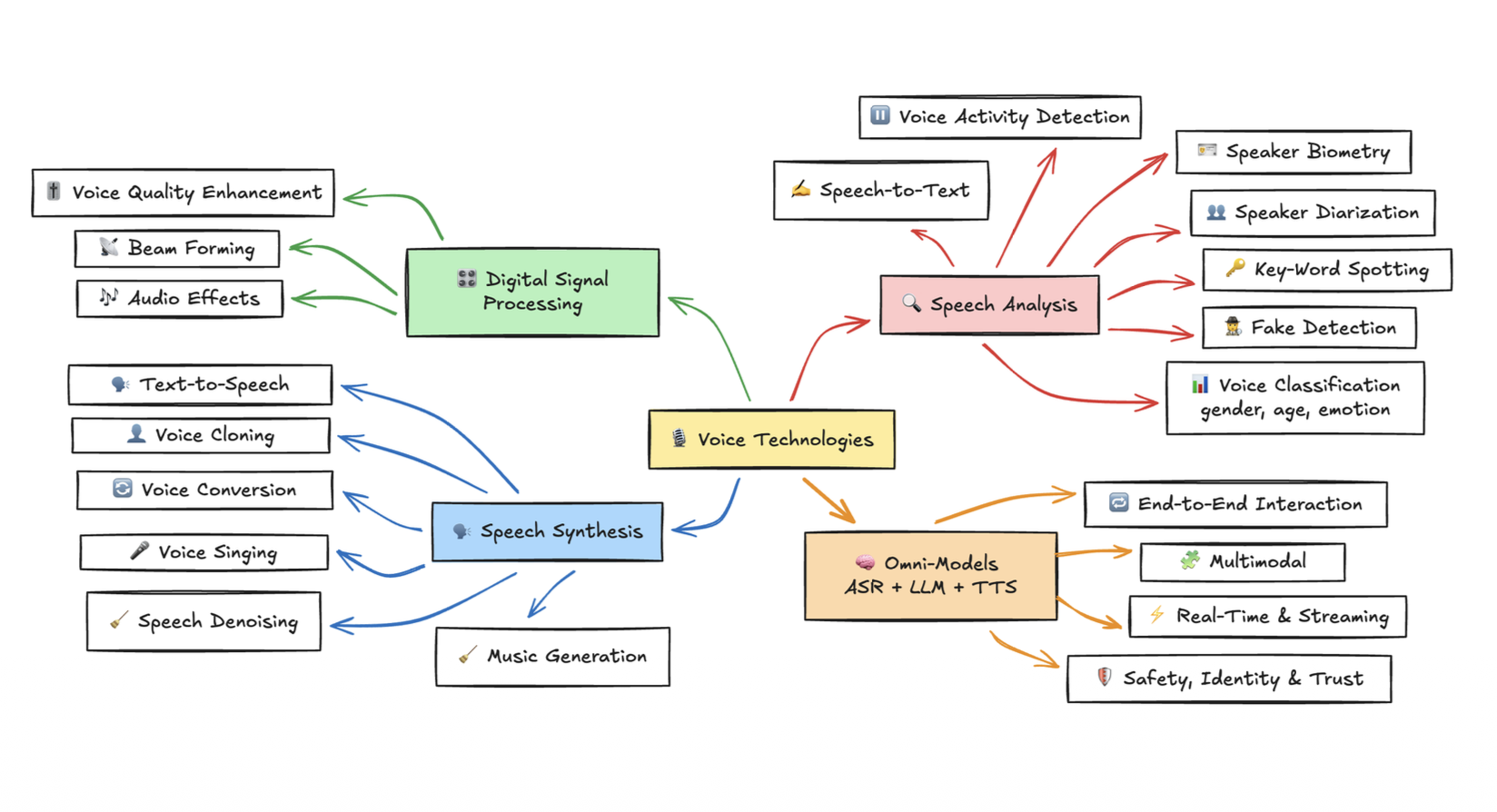
We can broadly group the tasks into speech analysis, speech synthesis, and larger systems. More specifically:
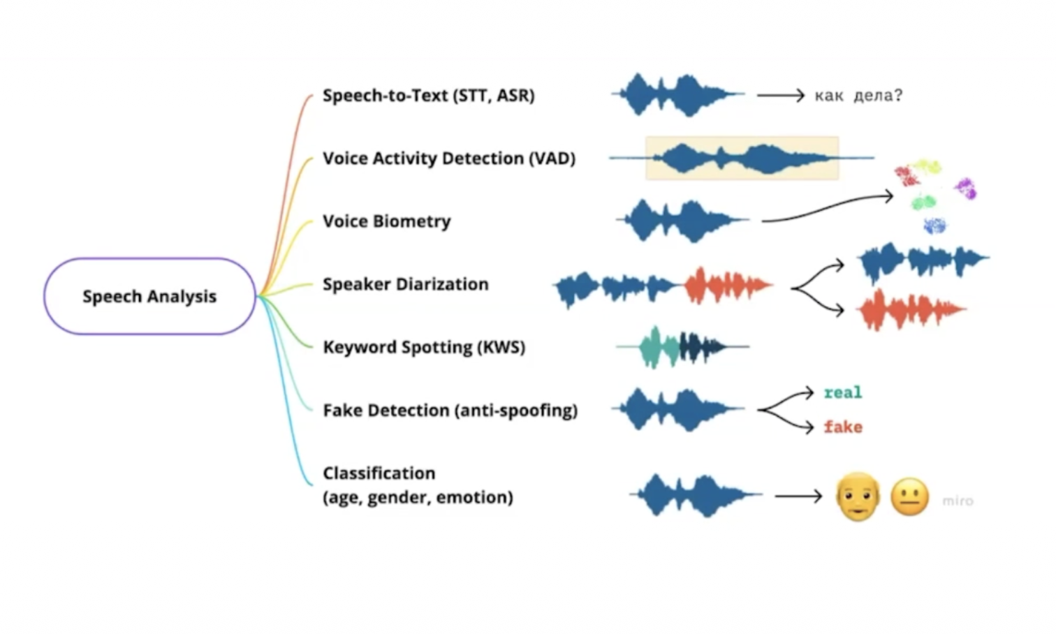
- Speech analysis
- ASR / Speech-to-Text: the classic speech recognition task. A traditional pipeline is raw audio → spectrogram → acoustic model → language model.
- VAD: detecting where someone is speaking. It is often used in voice assistant interactions, including detecting speech activity around wake-up and interruption.
- Speaker Recognition / Diarization: identifying a speaker or separating a conversation by speaker. Siri’s wake-up interaction can involve speaker identification.
- Keyword Spotting: detecting keywords, often for voice assistants.
- Fake Detection: detecting whether speech was generated by AI.
- Emotion / age / gender classification.
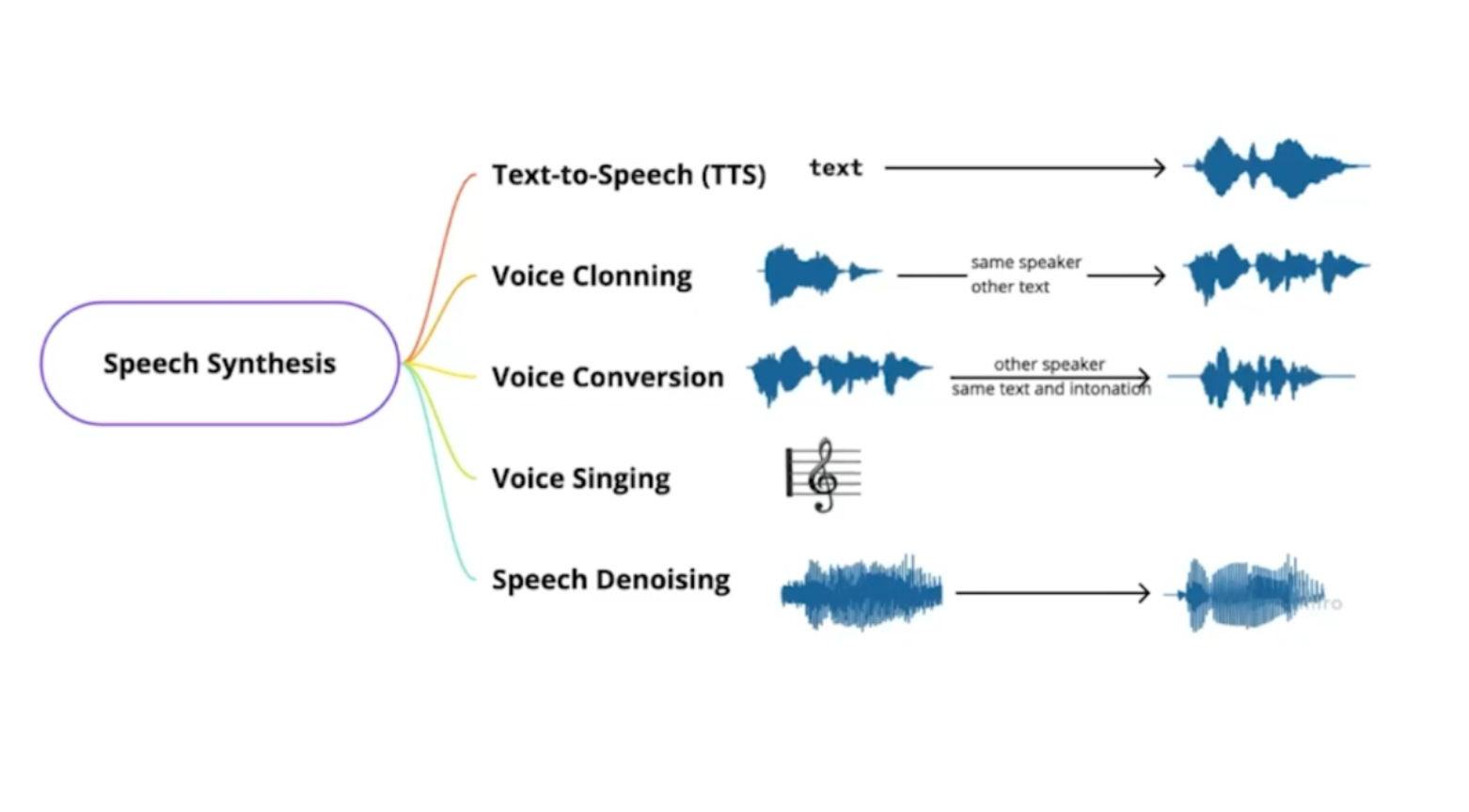
- Speech synthesis
- TTS: generating speech from text.
- Voice Cloning: cloning a voice from reference audio, for applications such as voice changers and AI voiceovers.
- Voice Conversion: changing one person’s voice into another’s while preserving the other aspects of the speech.
- Singing: exactly what it sounds like.
- Denoising: removing noise from speech input, such as Discord’s Krisp noise suppression.
- Larger systems
- Audio-to-audio conversation.
- Multimodal interaction.
- Real-time streaming.
What sound actually is
Physically, sound is a mechanical wave. In air, it travels through compression and rarefaction. If we plot the pressure at a fixed location over time, we get a waveform. The waveform is a measurement of how sound pressure changes over time at one location.
The cochlea in the human ear acts as a kind of spectrum analyzer. It coils like a snail shell, and different positions have different mechanical properties that make them respond to different frequencies. Hair cells at these positions convert mechanical vibrations into neural signals, which travel through nerves to the brain.
Sound in the real world is continuous, but we cannot measure or store every point. Instead, we sample at regular intervals. If we take one sample every 1/t seconds, the sample rate is t Hz. Once decoded, a mono audio recording is essentially a sequence of n numbers, where n = sample rate × duration. Multichannel audio has one such sequence per channel.
Different tasks need to preserve different maximum frequencies. Human hearing can typically extend to around 20 kHz, but ASR does not always need the full audible frequency range, so it often uses a sample rate of 16,000 Hz. This preserves frequencies below approximately 8 kHz. To preserve sound approaching 20 kHz, we need a higher sample rate. The Nyquist theorem states that, for a band-limited signal, the sample rate must be greater than twice the highest frequency we want to preserve: fs > 2 f_max.
The intuition is this: if all I see is a set of discrete sample points, how do I know what the original continuous wave looked like? After sampling, different continuous frequencies can produce exactly the same samples. The sample rate needs to be high enough to avoid that ambiguity.
Once we know that sound can be represented as a waveform, we can store the same waveform in different formats. WAV and AIFF commonly store uncompressed PCM data and often appear in audio deep learning. They are container formats and can also hold other encodings. FLAC and ALAC use lossless compression, so we can recover the original sample sequence. MP3, AAC, and Opus use lossy compression, trying to discard information that humans are less sensitive to.
Fourier transforms
We now have a list describing the strength of the sound wave at different times. But often, what we really want to know is: which frequencies are present, and how strong is each one?
Sounds in nature are generally combinations of many waves, so this is hard to see just by looking at the waveform. A Fourier transform compares our waveform with “standard waves” at different frequencies to see how well they match. For a complex audio recording, it can tell us how strong the 500 Hz component is, how strong the 501 Hz component is, and so on.
I recommend these two videos. I might write a separate post explaining this in more detail later:
A Fourier transform tells us which frequencies occur in a recording, but it does not tell us when they occur. A transform of the entire recording loses that time localization.
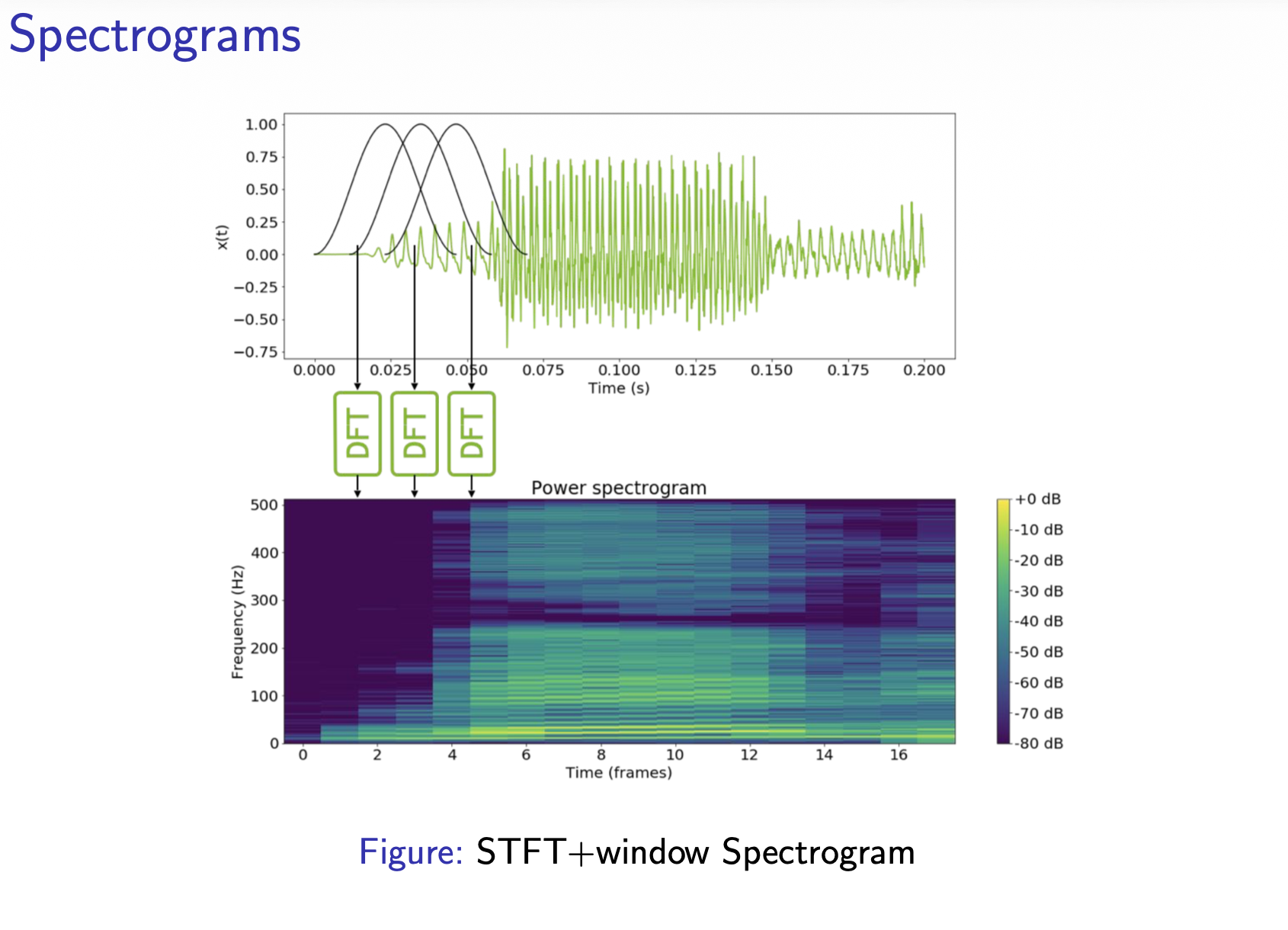
To bring time back in, we split the waveform into many short windows and apply a Fourier transform to each window separately. We get a representation indexed by frequency and time. This is the short-time Fourier transform (STFT); visualizing its magnitude or power gives us a spectrogram.
Mel spectrograms and MFCCs
An ordinary spectrogram has a linearly spaced frequency axis, but human frequency perception is not linear. The Mel scale maps frequencies from physical Hz to a representation closer to human hearing. The intuition is that, since speech tasks ultimately relate to human speech and hearing, we should allocate more representational resolution to the frequency regions where our ears are more sensitive.
At low frequencies, humans are more sensitive to frequency differences, so we want finer resolution. At high frequencies, the same difference in Hz is less perceptually noticeable, so we can compress that region.
MFCCs apply another transformation to a Mel spectrogram, compressing it into a more compact set of features that tends to describe the shape of the vocal tract. First, we take the logarithm: human loudness perception is approximately logarithmic, and this also turns source × filter into addition. Then we apply the DCT, using cosine basis functions to represent the original log-Mel values. This rearranges the information so that the smooth, large-scale spectral shape is concentrated in the first few coefficients.
A Mel spectrogram describes which frequency bands are present at each time, on a scale closer to human hearing. After log + DCT + truncation, we have a small number of coefficients summarizing the spectral shape or envelope of each frame.
For more on sampling rates and audio formats, see MDN’s digital audio concepts. For MFCC computation, see the TorchAudio documentation.