In the previous post, we introduced a framework for understanding ASR:
ASR = Representation + Alignment + Language + Knowledge + Deployment
This post continues with Alignment: how does continuous sound map to discrete text? I recommend reading the discussion of speech representations first.
Alignment: why do sound and text not line up?
An utterance may contain thousands of acoustic frames but only a few dozen characters or subword tokens. Training transcripts usually do not tell us how long each sound lasts or which frame should emit each token. Speaking the same sentence faster or slower changes that correspondence.
Here, alignment primarily means the mechanism connecting acoustic time to output symbols inside a recognition model. It relates to user-facing word timestamps, but the two are distinct: correct transcription does not automatically provide accurate word boundaries.
DTW: stretching and compressing the time axis
One route in early isolated-word recognition compared input acoustic features with recorded word templates and selected the closest match. Dynamic Time Warping (DTW) uses dynamic programming to accommodate differences in speaking rate.
For feature sequences of m and n frames, construct an m × n distance matrix. Each entry measures the distance between two feature vectors. Under boundary, monotonicity, and step constraints, find a path with minimum accumulated cost. A local stretch of one sequence can correspond to more or fewer frames of the other.
DTW directly aligns two acoustic feature sequences, rather than mapping frames to characters. The template supplies the word label; monotonicity preserves the temporal order of the sounds. Vector Quantization (VQ) can compress or discretize features, but it is not required by DTW.
DTW typically selects one optimal path instead of summing probabilities over alternatives. Ambiguous sound boundaries motivate a different approach: treat alignment as a latent variable.
HMMs: probabilistic alignment paths
Hidden Markov Models (HMMs) were central to traditional ASR. Consider cat as /k/, /æ/, /t/: the order is known, but the frame durations are not.
For illustration, assign one state to each phoneme, with self-loops and forward transitions:
/k/ → /æ/ → /t/
 ↺     ↺     ↺
Two possible paths through eight frames are:
Path A: k, k, æ, æ, æ, t, t, t
Path B: k, æ, æ, æ, æ, t, t, t
Path A assigns x₁–x₂ to /k/, x₃–x₅ to /æ/, and x₆–x₈ to /t/. Path B gives /k/ a shorter duration. Real recognizers often use multiple states per phoneme and context-dependent, tied states.
Forward-Backward computes state and transition posteriors; Baum-Welch / EM uses them to update parameters without fixing one path in advance. Viterbi decoding selects the highest-scoring path, with practical recognition also incorporating a lexicon and language model. A useful shorthand is sum over paths during training; maximize over paths during Viterbi decoding, although other HMM training and decoding strategies exist.
From GMM-HMM to DNN-HMM
Neural networks did not immediately eliminate HMMs. DNN-HMM systems changed the acoustic scores while retaining the HMM alignment and transition framework.
A GMM models the observation likelihood p(xₜ | qₜ). A typical hybrid DNN instead predicts state posteriors P(qₜ | x), potentially using multiple frames of context. During decoding, dividing the posterior by the state prior P(qₜ) gives a score proportional to the acoustic likelihood through Bayes’ rule. The DNN therefore does not simply replace the GMM with an identical kind of probability output.
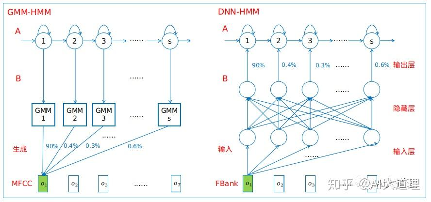
Image from the original note, with its watermark preserved. MFCC and FBank are example frontends, not mandatory features for these frameworks.
On this route, deep learning initially changed Representation / Acoustic Modeling rather than removing Alignment.
CTC: summing paths that produce the target text
End-to-end ASR aims to reduce reliance on hand-designed phoneme states and pronunciation lexicons, but still needs to connect 1,000 acoustic frames with 20 text tokens. Connectionist Temporal Classification (CTC, 2006) provides a training objective without frame-level labels.
At each encoder time step, CTC predicts a vocabulary token or blank. Its collapse mapping first merges consecutive repeated symbols, then removes blanks:
c c _ a a _ t → c _ a _ t → catBlank means no text emission at that step, rather than simply silence. It can separate repeated characters: l _ l retains two l’s, while l l becomes one.
Let X be audio, Y the target text, A a framewise path, and B the collapse mapping:
P(Y | X) = Σ over A with B(A) = Y of P(A | X)
P(A | X) = ∏ₜ P(aₜ | X)
CTC loss = −log P(Y | X)
Dynamic programming performs the sum efficiently. Output units can be characters, subwords, or phonemes. CTC defines both a monotonic alignment mechanism and a differentiable loss.
Conditional independence does not mean no acoustic context
CTC factorizes path probabilities across time given X, without explicitly conditioning on previously emitted text. An external language model can supply output dependencies.
However, a BiLSTM or global-attention encoder may compute P(aₜ | X) using the full recording. Streaming also requires a causal encoder or limited lookahead, plus appropriate decoding and output commitment policies. CTC alone does not guarantee it.
LAS / AED: learning where to attend
Listen, Attend and Spell (LAS, 2015) is an Attention-based Encoder-Decoder (AED). It forms acoustic context through soft attention rather than summing discrete monotonic paths using CTC’s blank-collapse rule.
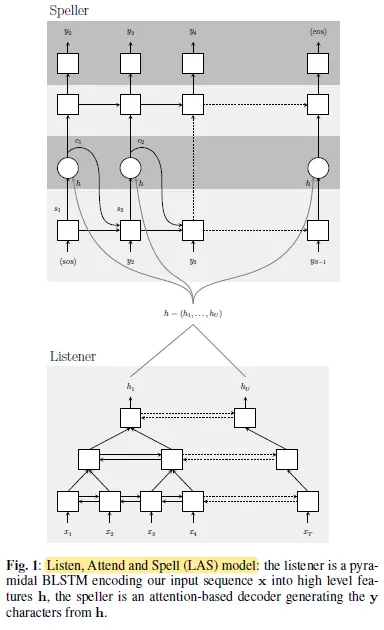
Image from the original note, corresponding to Figure 1 of the LAS paper.
Its operation has three parts:
- Listen: a pyramidal BiLSTM encodes filter-bank features into a shorter sequence of representations h.
- Attend: the decoder state and encoder representations determine attention weights and a weighted acoustic context.
- Spell: the decoder predicts the next character using that context and previously generated characters.
Text probability has an autoregressive factorization:
P(Y | X) = ∏ᵤ P(yᵤ | y<ᵤ, X)Original LAS needs the full input because of its bidirectional encoder and full-input attention. Soft attention does not enforce rightward movement, and its weights do not automatically provide reliable word boundaries.
This does not apply to every AED: monotonic attention, chunk attention, and streaming encoders can limit future information. Streaming depends on the model and system design, rather than the mere presence of attention.
RNN-T: monotonic alignment with output history
Recurrent Neural Network Transducer (RNN-T) conditions predictions on acoustic input and previous outputs while summing over legal monotonic paths. It appeared in 2012, before LAS. It should not be described as a later fix for LAS; CTC, RNN-T, and AED are coexisting approaches.
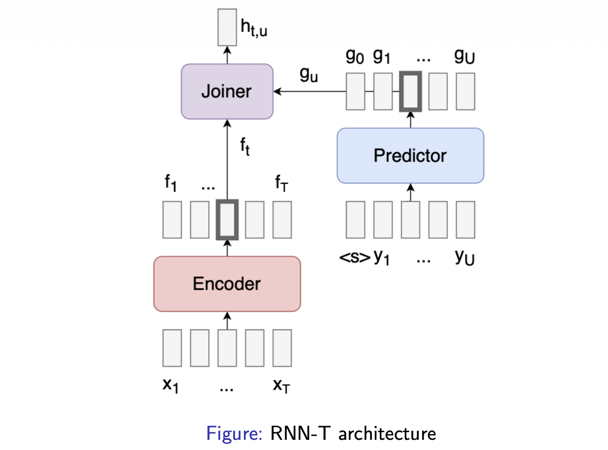
RNN-T architecture illustration supplied in the original note.
The encoder produces hₜ from audio. The predictor produces gᵤ from preceding non-blank tokens. The joiner combines them to predict a token or blank:
P(k | t, u, X, y≤ᵤ) = softmax(joiner(hₜ, gᵤ))[k]On a lattice with encoder time and output position as its axes, T counts encoder steps and U counts target tokens:
- A regular token advances u while keeping t fixed.
- Blank advances t while keeping u fixed.
Several tokens can therefore be emitted at one acoustic step. Training sums paths that produce the target; decoding uses greedy or beam search, among other strategies.
Streaming still requires an encoder restricted to available audio or bounded future context. Modern encoders can use streaming Transformers or Conformers despite the RNN-T name.
Computational tradeoffs in deployment
One RNN-T bottleneck is sequential decoding: each emitted token updates the predictor, and acoustic time typically advances after blank. Standard full-lattice training also involves roughly T × (U + 1) positions, motivating approaches such as pruning to reduce memory and computation.
When T greatly exceeds U, a standard alignment path contains T blank advances and U token emissions, so blank advances can dominate. This is not simply a consequence of silence: blank also advances time during speech. Actual GPU utilization depends on the encoder, batching, search, and implementation; it is too broad to call RNN-T GPU utilization inherently “extremely low.”
The following methods address different problems rather than forming one evolutionary chain:
| Method | Relationship to alignment | Core idea | Main goal |
|---|---|---|---|
| HAT | A transducer probability-modeling variant | Separately model blank probability and the non-blank label distribution, enabling internal LM estimation | More principled external language model fusion |
| TDT | Extends RNN-T | Jointly predict a token and duration, potentially advancing several encoder steps at once | Fewer decoding steps and faster inference |
| CIF | A soft, monotonic alignment mechanism | Integrate frame representations with learned weights; emit a token-level representation at a threshold | Connect continuous acoustic representations to discrete output positions |
| CTC + RNN-T Hybrid | Multiple objectives sharing an encoder | Use CTC and transducer heads / losses | Assist alignment learning and provide different decoding paths |
CIF firing positions should not automatically be treated as verified word boundaries. Hybrid benefits likewise depend on implementation and experiments.
Whisper: alignment becomes part of generation
Whisper uses a Transformer encoder-decoder with large-scale multilingual, multitask weak supervision, bringing transcription and translation into a shared generation framework.
Cross-attention connects audio with text, while learned timestamp tokens supply explicit segment timing. They do not provide CTC-style framewise monotonic alignment: the original timestamp resolution is 20 ms, which does not guarantee accurate word boundaries. Precise word timing may still require additional alignment methods.
Whisper demonstrates the power of training scale and task design, but it does not establish that AED or Audio-LLMs have unified offline ASR. AED describes a recognition model factorization; Audio-LLM refers to a broader family of model and system designs. The Whisper paper also discusses repetition loops, omissions, and hallucinations in long-form transcription; their severity should not be generalized to every attention model.
Practical choices involve recognition quality, throughput, latency, long-audio stability, and timing requirements. CTC’s framewise head permits parallel computation; transducers retain monotonic structure while using output history; AED supports flexible contextual modeling. Stronger output dependencies alone do not guarantee greater recognition accuracy.
Streaming ASR also cannot be divided into scenes supposedly “ruled” by one architecture. CTC, RNN-T / TDT, CTC + AED, and constrained-attention AED can all serve different systems. Chunk size, lookahead, endpointing, and output commitment affect latency too. Architectures provide tradeoffs; their advantages need evaluation under comparable data and deployment conditions.
Takeaways
Alignment has developed through changes in alignment constraints, output dependencies, and computational cost, rather than simple replacement.
DTW selects an acoustic template-matching path; HMMs make state paths probabilistic; CTC sums blank-collapse paths; RNN-T adds output history along monotonic paths; LAS / AED obtains acoustic context through attention.
Speech has a strong temporal ordering. Preserving that inductive bias can help streaming design and alignment stability; greater modeling freedom supports more flexible contextual reasoning. The final behavior still depends on the full ASR framework: Representation, Alignment, Language, Knowledge, and Deployment.