This post is part I of my explanation of ASR models. I assume readers have some familiarity with computer vision and NLP, so there is a bit of a prerequisite. ASR is already widely used across many fields. Its central job is to turn speech into text, with applications including:
| Scenario | Typical examples | What ASR does |
|---|---|---|
| Voice assistants / Voice agents | Siri, in-car assistants, AI customer service | Transcribes the user’s speech for an LLM or NLU system |
| Meeting / call transcription | Zoom, Teams, meeting notes | Produces transcripts in real time or offline |
| Subtitles | YouTube, live streams, courses | Generates live subtitles or closed captions |
| Customer service / Call centers | Support calls, sales calls | Transcribes calls for quality review, summarization, and intent analysis |
| Voice input | Phone dictation, voice search | Replaces keyboard input with speech |
| Audio and video search | Podcasts, interviews, video libraries | Produces text that can be indexed for search |
| Medical / legal records | Dictated clinical notes, court proceedings | Transcribes speech containing specialized vocabulary |
| Accessibility | Live captions for people with hearing loss | Displays surrounding speech as text in real time |
| Multimodal / Speech LLMs | Qwen-Omni, GPT-style voice systems | Provides a frontend or intermediate capability for speech understanding |
ASR applications and system modes
Based on whether the complete recording is available, we can distinguish two ASR operating modes:
- Offline ASR: the complete recording is already available, as with podcast or video subtitles. Accuracy is usually the priority, with less sensitivity to latency.
- Streaming ASR: speech arrives while the model produces output. Live captions and telephone customer service are common examples. Latency and continuity matter alongside accuracy.
Full-duplex speech interaction describes a broader interaction system that keeps listening while producing speech and handles interruptions and barge-in. ASR or speech understanding is one component of that system, rather than a third ASR mode alongside offline and streaming.
Evaluating ASR
Before getting into the principles and models, we should understand how to evaluate an ASR model. Model evaluation includes accuracy and robustness, but also latency, real-time factor (RTF: processing time divided by audio duration), memory use, streamability, and long-audio capability. System evaluation additionally considers overall throughput and end-to-end latency.
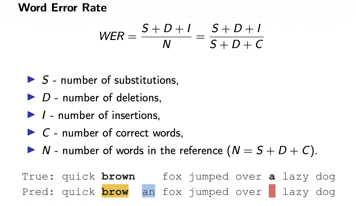
Levenshtein distance, or edit distance, asks: given two sequences a and b, usually a prediction and ground truth, what is the minimum number of edits needed to turn a into b? The allowed operations are substitution, insertion, and deletion, each with a cost of one. This is also a classic dynamic programming problem on LeetCode.
WER normalizes that edit distance by the number of words in the reference. CER works similarly, changing the basic unit from words to characters. WER is commonly used for languages with clear word boundaries, such as English. CER is commonly used for languages whose word boundaries are less explicit, such as Chinese and Japanese.
Common ASR datasets
| Dataset | Characteristics | Main use |
|---|---|---|
| LibriSpeech | English audiobooks, relatively clean audio | A classic benchmark |
| Common Voice | Crowdsourced, multilingual, short utterances | Multilingual ASR |
| GigaSpeech | Podcasts, YouTube, spontaneous speech | Conditions closer to real-world audio |
| Earnings-22 | Earnings calls | Accents and business speech |
| AMI | Meetings | Spontaneous meeting ASR |
| FLEURS | 102 languages | Multilingual and zero-shot evaluation |
Challenges that remain
Even with low WER on benchmarks, modern ASR still faces many challenges.
Acoustic ambiguity: the same sentence can sound very different, and different content can sound similar.
- Noise: background music, street noise, and keyboard sounds interfere with the speech signal.
- Accents: people from different regions and native-language backgrounds may pronounce the same word very differently.
- Overlapping speakers: when two people talk at once, the model needs to separate and recognize their speech from a mixture.
- Far-field speech: distance from the microphone introduces attenuation, reverberation, and echoes that blur speech features.
Linguistic ambiguity: even when the sound is clear, pronunciation alone may not determine the correct text.
- Homophones and near-homophones: context is needed to distinguish words that sound identical or similar.
- Personal names, place names, and proper nouns: these may be rare or unseen during training.
- Domain terminology: medicine, law, finance, and technology contain many uncommon terms that are difficult to recognize from acoustics alone.
Long audio and contextual dependencies: recognizing the current utterance often requires a broader context.
- Earlier context affects later interpretation: the same pronunciation may correspond to different words in different contexts.
- Punctuation and segmentation: ASR systems often also need to determine pauses, sentence boundaries, and punctuation.
- Speaker turns: meeting and conversation systems need to identify when the speaker changes.
Streaming constraints: the model must start producing results before the utterance has ended.
- Future audio is unavailable: only audio received so far can be used.
- Latency versus accuracy: waiting provides more context and often improves accuracy, but makes the system less responsive.
Five perspectives on ASR
To make ASR easier to understand, I will explain its development and the ideas behind it through five perspectives. I personally find the original AI Audio Masters slides a little jumpy: they do not quite explain how ASR arrived where it is today. So I will use a framework I worked out through some back-and-forth with GPT. This post covers representation; the next post will continue with the other parts.
ASR = Representation + Alignment + Language + Knowledge + Deployment
| Dimension | Central question |
|---|---|
| Representation | How should sound be represented? |
| Alignment | How does continuous audio correspond to discrete text? |
| Language | Which text sequence is more plausible? |
| Knowledge | Where does the model learn these capabilities? |
| Deployment | Under what real-world constraints must the model run? |
Representation: from handcrafted features to learned representations
As a quick recap, the previous post explained how sampling turns a sound wave into a long list of digital values. Early ASR often relied on manually designed features, transforming the waveform into a spectrogram and then into MFCCs. Another common representation in speech processing is Fbank, or filterbank features, which in this context means log-Mel features.
These choices already build in a lot of knowledge about speech. MFCCs try to retain information about the sounds someone produced while reducing less relevant spectral details. They are a typical handcrafted representation. Although MFCCs are no longer the mainstream choice, they reflect what we want from a good ASR representation: preserve linguistic information while discarding nuisance information, such as microphone noise and background interference.
As deep learning developed, we increasingly wanted models to learn hidden representations themselves, much as in computer vision, instead of relying entirely on expert-designed features.
CNNs and RNNs: different inductive biases
This is not a linear history of CNN → RNN/LSTM → Transformer. RNNs and LSTMs were widely used in ASR before pure convolutional models such as QuartzNet; for example, Deep Speech used RNNs in 2014. CNNs favor local acoustic structure, while RNNs and LSTMs accumulate temporal context. These complementary inductive biases are also often combined.
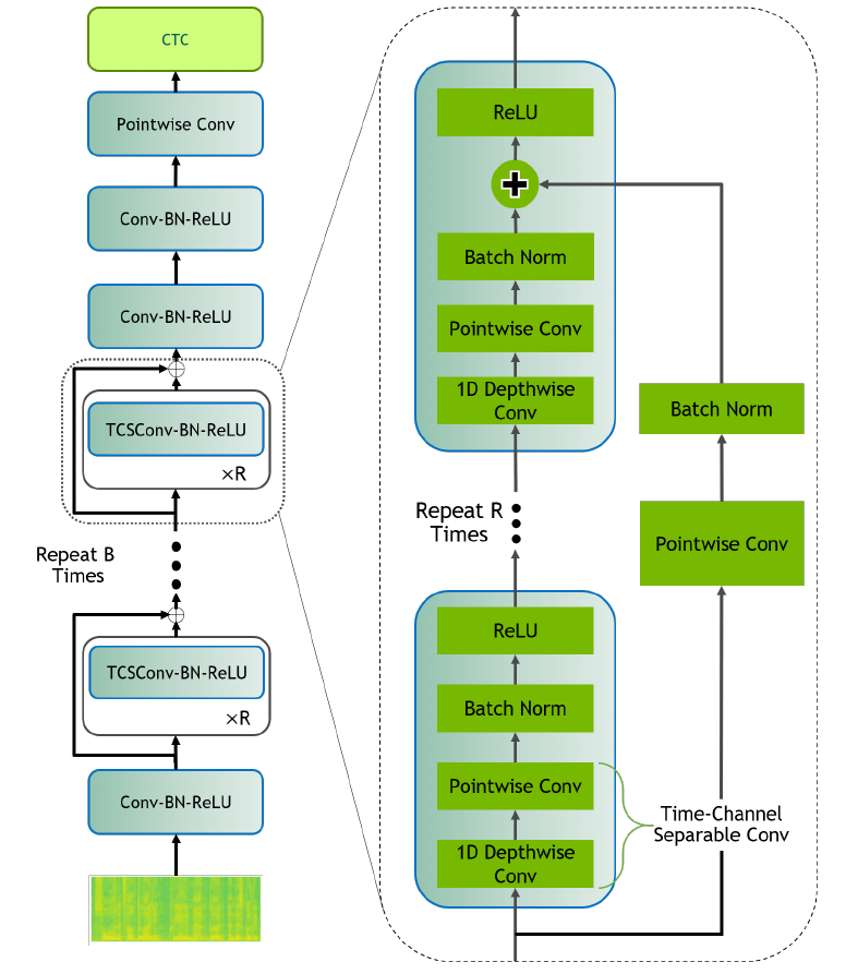
CNNs were a natural choice because speech has clear local structure. NVIDIA’s QuartzNet is a classic ASR architecture built around a convolutional encoder. Notice that it convolves along time and takes a Mel-scale spectrogram as input rather than MFCCs.
RNNs, LSTMs, and Transformers: temporal context
Speech is fundamentally a long sequence, and RNNs and LSTMs model temporal context through recurrent states. Transformers later introduced self-attention to model relationships between positions. In a non-streaming setting with global attention, each position can directly attend to the entire sequence.
A unidirectional RNN or LSTM only sees the current input and earlier information. Bidirectional architectures such as BiLSTMs also incorporate future context. However, recurrent models face two major difficulties:
- Sequential dependencies: the next state depends on the previous one, making training hard to parallelize fully along time. This is a poor fit for modern GPUs. Transformers allow much more parallel computation.
- Long information paths: information from h1 to h1000 travels through roughly a thousand recurrent steps. Self-attention can directly connect two positions in a sequence.
Although NLP quickly embraced Transformers, speech representation did not stop at the vanilla Transformer. Text is already highly compressed: a sentence might have only 20 tokens. Audio is dense: a minute can contain around 6,000 frames. That is expensive for vanilla self-attention, whose complexity is O(T²).
Conformer: local structure and global context
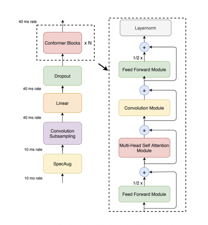
An important development was Conformer, one of the major Transformer variants for ASR. It combines Transformers and CNNs because speech contains both local acoustic patterns and global context. Formants, phoneme transitions, and transients over tens of milliseconds are local patterns; words, sentences, and longer context also require broader modeling.
Self-supervised representations and acoustic frontends
Self-supervised learning developed alongside architecture design. Conformer and wav2vec 2.0 both appeared in 2020, but address different questions: architecture and learning representations from unlabeled audio. Supervised ASR representation learning relies on paired audio and text; methods like wav2vec 2.0 showed that large amounts of audio without transcripts could first be used to learn representations. A model learns through masked prediction and a contrastive objective, then is fine-tuned on labeled ASR data. Representation learning becomes less tightly coupled to specific ASR labels.
Modern models have not abandoned handcrafted representations entirely. Whisper still uses log-Mel spectrograms rather than raw waveforms. Models take on more of the representation learning, but a cheap, stable acoustic frontend with a useful inductive bias can still be valuable. Mel frontends remain common in ASR.
Efficiency and deployment-driven architecture: FastConformer
Conformer is powerful, but full attention remains expensive. FastConformer, published in 2023, addresses efficiency and deployment constraints by reducing the number of time steps processed downstream. Its depthwise separable convolutional subsampling reduces the input sequence length by a factor of eight, greatly reducing the later attention workload. The work also explores Longformer-style attention with local windows and global tokens for efficient modeling of long recordings.
Connections across modalities and architecture choices
There is a related point here: representations across modalities influence one another. Early computer vision, audio, and NLP largely handled their own inputs separately: two-dimensional pixels, continuous waveforms or spectrograms, and discrete tokens.
ASR later borrowed heavily from computer vision. A spectrogram is a two-dimensional time-frequency map, so CNNs were a natural fit. Their strength in local patterns matches speech well. QuartzNet and earlier convolutional acoustic models share ideas with the feature hierarchies used in vision.
CNNs and RNNs should not be understood simply as one replacing the other. They approach modeling from different directions. As NLP grew, RNNs and LSTMs were natural in both NLP and ASR because both involve sequences. The inputs differ: NLP starts with discrete tokens, while ASR starts with dense, continuous frames.
Transformers marked a major point of convergence. They first took off in NLP, then spread to vision and speech. Their abstraction is broadly reusable: turn a modality into a sequence of vectors, then apply self-attention. This gave us BERT and GPT in NLP, ViT in vision, and Transformer encoders, Conformer, and Whisper in speech. The underlying idea is to tokenize, patchify, or encode each modality into vectors, then model context.
Speech’s dependence on local structure is one reason vanilla Transformers were not the final answer. Conformer restores explicit local modeling through convolution, much like hybrid architectures in vision. It is an important specialization of Transformers for speech and audio.
Transformer and Conformer architectures coexist, and either can be designed for streaming or non-streaming operation. Streaming is an operating constraint, not a separate architecture category. Convolution’s explicit modeling of local acoustics is useful in dedicated and streaming ASR. Pure Transformers are broadly reusable and can be convenient to scale, especially in speech encoder + LLM systems and multimodal foundation models. Edge devices, streaming, high throughput, and large multimodal systems have different goals, so they do not share a single optimal architecture.